Lab 12 — PPP2R2B expression and isoforms
Time: ~55 min · Before this: Ch 47–48 · lab-06 · lab-09 · D4 SCA12 I
Statistics used here: S3 Sampling and estimation · S4 Hypothesis testing
D4 leaves you holding five candidate mechanisms for and no winner. The oldest of them — Hypothesis A, that the expanded CAG tract acts as a cis element raising output until the cannot cope — makes a prediction that sounds testable from public data alone: if the disease is a dosage disease of the cerebellum, PPP2R2B should look like a cerebellar gene. In this lab you go and find out. Three descents in resolution — whole tissue, transcript, single nucleus — each answering a sharper version of the question, each running on a laptop from open-access files. Every number below was produced on this machine, and the answer to the headline question is no, which is far more interesting than yes would have been.
The lab leans on medians, proportions and small-sample uncertainty, and assumes none of it. Boxes marked The statistics here say what the printed number assumes and point at the statistics chapter that derives it — S3 for estimators and sampling error, S4 for what a comparison can and cannot conclude.
# GENOMICS is exported in lab-00. In a fresh shell, set it again:
#   export GENOMICS=/path/to/learn-genomics
cd "$GENOMICS" && source .venv/bin/activate && cd labs/data
uv pip install scanpy
Tool note. Everything here is curl plus the Python stack lab-06 and lab-09 already installed; the uv pip install scanpy line is a no-op if you have done lab-09. Versions used here: pandas 3.0.5, numpy 2.5.2, matplotlib 3.11.1, scanpy 1.12.3, anndata 0.13.2. No genome, no aligner, no index. Total download for the whole lab: 8.8 MB + 431 MB + 164 MB ≈ 604 MB, of which the two single-cell files are §4 and are optional if your laptop is short of memory — the fallback in §4 keeps the argument intact.
1. Write the hypothesis down as a measurement
Before touching a file, commit to what would count as evidence. Hypothesis A, as D4 states it, is a chain: the expanded repeat sits in the 5′ region of , raises of the repeat-bearing transcript, and the extra B55β poisons cerebellar neurons. Three links, and public expression data from healthy donors can only speak to the background conditions of the third.
| What Hypothesis A needs | What open expression data can say | Where in this lab |
|---|---|---|
| The gene is expressed in the tissue that degenerates | Directly measurable | §2 |
| It is expressed there preferentially — enough for a dosage change to bite there and nowhere else | Directly measurable, and this is the load-bearing claim | §2, §4 |
| The repeat sits in the transcript that dominates that tissue | Measurable at transcript level, with caveats | §3 |
| The cells that die express it | Needs single-cell resolution | §4 |
| The expanded raises output | Not measurable here at all — every donor in these datasets is a control | §5 |
Notice the shape of that table. The last row is the hypothesis; the rest are its preconditions. A lab that can only test preconditions can falsify by knocking one out, and can never confirm. That asymmetry is the whole design, and §5 is where you have to be honest about it.
The prediction to write on a sticky note now, before you have the answer: if is a cerebellar dosage disease, then PPP2R2B median expression in should exceed other brain regions, and should be concentrated in the cerebellar neurons that die.
2. Tissue level: is PPP2R2B cerebellum-enriched? ★
GTEx v10 publishes one small file that answers this: the median of every gene in every tissue. 8.8 MB, no registration, no API key.
curl -sL -O https://storage.googleapis.com/adult-gtex/bulk-gex/v10/rna-seq/GTEx_Analysis_v10_RNASeQCv2.4.2_gene_median_tpm.gct.gz
ls -l GTEx_Analysis_v10_RNASeQCv2.4.2_gene_median_tpm.gct.gz
-rw-r--r-- 1 user staff 8846936 GTEx_Analysis_v10_RNASeQCv2.4.2_gene_median_tpm.gct.gzTwo ways to misread the file, both worth hitting
Read it the obvious way first:
python -c "
import pandas as pd
d = pd.read_csv('GTEx_Analysis_v10_RNASeQCv2.4.2_gene_median_tpm.gct.gz', sep='\t')
print(d.shape)
"
pandas.errors.ParserError: Error tokenizing data. C error: Expected 2 fields in line 3, saw 70That is the GCT format announcing itself. A .gct is a TSV with a two-line preamble: line 1 is a version string (#1.2), line 2 is <n_rows>\t<n_cols>, and the real header is line 3. Pandas saw a two-field line 2, decided the table had two columns, then met 70 fields. Skip the preamble and it parses:
python - <<'PY'
import pandas as pd
d = pd.read_csv('GTEx_Analysis_v10_RNASeQCv2.4.2_gene_median_tpm.gct.gz', sep='\t', skiprows=2)
print('genes x columns:', d.shape[0], 'x', d.shape[1]-2)
print('rows whose Name is exactly ENSG00000156475:',
      int((d.Name == 'ENSG00000156475').sum()))
print('rows whose Name starts with it            :',
      int(d.Name.str.startswith('ENSG00000156475').sum()))
print('the value actually stored                 :',
      d.loc[d.Name.str.startswith('ENSG00000156475'), 'Name'].item())
PY
genes x columns: 59033 x 68
rows whose Name is exactly ENSG00000156475: 0
rows whose Name starts with it : 1
the value actually stored : ENSG00000156475.19A gene ID without its version is not the ID in the file. is
ENSG00000156475, and GTEx v10 storesENSG00000156475.19— the GENCODE version suffix that increments whenever the gene model is revised. An exact-match join returns zero rows and no error, which in a pipeline reads as "the gene is not expressed" rather than "your key was wrong". Either strip the suffix on both sides or match on theDescriptionsymbol column, and never let a lookup that returns nothing pass silently.
The answer
68 columns is not 68 tissues: 54 are primary tissues and 14 are laser-capture sub-columns (Liver_Hepatocyte, Pancreas_Islets, Stomach_Mucosa and so on) that would double-count their parent organ. Drop them, then rank.
python - <<'PY'
import pandas as pd, numpy as np
LCM = ['Colon_Transverse_Mixed_Cell','Colon_Transverse_Mucosa','Colon_Transverse_Muscularis',
       'Liver_Hepatocyte','Liver_Mixed_Cell','Liver_Portal_Tract','Pancreas_Acini',
       'Pancreas_Islets','Pancreas_Mixed_Cell',
       'Small_Intestine_Terminal_Ileum_Lymphode_Aggregate',
       'Small_Intestine_Terminal_Ileum_Mixed_Cell','Stomach_Mixed_Cell','Stomach_Mucosa',
       'Stomach_Muscularis']
d = pd.read_csv('GTEx_Analysis_v10_RNASeQCv2.4.2_gene_median_tpm.gct.gz', sep='\t', skiprows=2)
X = d.set_index('Description').iloc[:, 1:].astype(float).drop(columns=LCM)
X.to_csv('gtex_v10_primary.tsv', sep='\t')     # the rest of §2 reuses this
row   = X.loc['PPP2R2B']
brain = [t for t in X.columns if t.startswith('Brain')]
other = [t for t in X.columns if not t.startswith('Brain')]
print('primary tissues:', X.shape[1], ' brain columns:', len(brain))
print(row[brain].sort_values(ascending=False).round(2).to_string())
print('\nmedian across the %d non-brain tissues: %.3f' % (len(other), np.median(row[other])))
print('cerebellum / median non-brain          : %.1f x' % (row['Brain_Cerebellum']/np.median(row[other])))
print('frontal cortex BA9 / cerebellum        : %.2f x' % (row['Brain_Frontal_Cortex_BA9']/row['Brain_Cerebellum']))
PY
primary tissues: 54 brain columns: 13
Brain_Frontal_Cortex_BA9 29.71
Brain_Nucleus_accumbens_basal_ganglia 26.62
Brain_Cortex 24.80
Brain_Caudate_basal_ganglia 21.52
Brain_Anterior_cingulate_cortex_BA24 21.17
Brain_Putamen_basal_ganglia 18.06
Brain_Amygdala 16.70
Brain_Hypothalamus 15.10
Brain_Substantia_nigra 14.43
Brain_Hippocampus 13.63
Brain_Spinal_cord_cervical_c-1 13.47
Brain_Cerebellum 10.02
Brain_Cerebellar_Hemisphere 8.78
median across the 41 non-brain tissues: 0.520
cerebellum / median non-brain : 19.3 x
frontal cortex BA9 / cerebellum : 2.97 xRead that ranking carefully, because it kills a story most reviews of still carry. PPP2R2B is emphatically brain-enriched — 19× the median non-brain tissue, and roughly 1,000× cultured fibroblasts. And the two cerebellar columns are the two lowest brain regions in the list. Frontal cortex carries three times as much. Whatever explains a cerebellar , it is not that the is where this gene lives.
How enriched is "enriched"? Put it against every gene
"Cerebellum is 12th of 13" is a rank; it does not say how far from cerebellar-specific the gene is. Score every expressed gene the same way — cerebellum against its best non-cerebellar tissue — and read PPP2R2B's position in that distribution.
python - <<'PY'
import pandas as pd, numpy as np
X  = pd.read_csv('gtex_v10_primary.tsv', sep='\t', index_col=0)
CB = 'Brain_Cerebellum'
expr  = X[X.max(axis=1) >= 5]                                  # a gene must be on somewhere
num   = expr[CB].clip(lower=0.1)                               # floor both sides: 0/0 is not a ratio
den   = expr.drop(columns=[CB, 'Brain_Cerebellar_Hemisphere']).max(axis=1).clip(lower=0.1)
ratio = num / den
print('genes scored:', len(ratio), '  median gene ratio: %.3f' % ratio.median())
print('genes with ratio > 5 (cerebellum-enriched by any reasonable reading):', int((ratio > 5).sum()))
for g in ['GABRA6', 'CBLN3', 'CALB1', 'PPP2R2A', 'PPP2R2B']:
    print(f'  {g:8s} ratio {ratio[g]:8.2f}   rank {int((ratio > ratio[g]).sum())+1:6d}')
PY
genes scored: 22948 median gene ratio: 0.194
genes with ratio > 5 (cerebellum-enriched by any reasonable reading): 144
GABRA6 ratio 275.46 rank 1
CBLN3 ratio 35.18 rank 21
CALB1 ratio 1.24 rank 1443
PPP2R2A ratio 0.35 rank 8692
PPP2R2B ratio 0.34 rank 8947Plot both halves — the profile, and the profile's place in the reference distribution:
python - <<'PY'
import pandas as pd, numpy as np, matplotlib
matplotlib.use('Agg'); import matplotlib.pyplot as plt
X  = pd.read_csv('gtex_v10_primary.tsv', sep='\t', index_col=0)
row, CB = X.loc['PPP2R2B'], 'Brain_Cerebellum'
brain = [t for t in X.columns if t.startswith('Brain')]
expr  = X[X.max(axis=1) >= 5]
ratio = (expr[CB].clip(lower=0.1)
         / expr.drop(columns=[CB, 'Brain_Cerebellar_Hemisphere']).max(axis=1).clip(lower=0.1))

fig, ax = plt.subplots(1, 2, figsize=(12.5, 5.2))
sel = brain + ['Nerve_Tibial','Pituitary','Testis','Whole_Blood','Liver','Muscle_Skeletal',
               'Cells_Cultured_fibroblasts']
v = row[sel].sort_values()
ax[0].barh(range(len(v)), v.values,
           color=['#c0392b' if t.startswith('Brain_Cerebell') else
                  '#2e6da4' if t.startswith('Brain') else '#9e9e9e' for t in v.index])
ax[0].set_yticks(range(len(v)))
ax[0].set_yticklabels([t.replace('Brain_','').replace('_',' ') for t in v.index], fontsize=8)
ax[0].set_xscale('log'); ax[0].grid(axis='x', alpha=.3)
ax[0].set_xlabel('PPP2R2B median TPM (GTEx v10, log scale)')
ax[0].set_title('Brain-enriched — and the two cerebellar columns are the lowest brain regions', fontsize=9.5)

ax[1].hist(np.log10(ratio), bins=90, color='#bdbdbd')
for gene, c in [('PPP2R2B','#c0392b'), ('CALB1','#2e6da4'), ('GABRA6','#1b7837')]:
    ax[1].axvline(np.log10(ratio[gene]), color=c, lw=2)
    ax[1].text(np.log10(ratio[gene]), ax[1].get_ylim()[1]*.95, ' '+gene,
               color=c, fontsize=8, rotation=90, va='top')
ax[1].axvline(0, color='k', ls=':', lw=1); ax[1].grid(alpha=.3)
ax[1].set_xlabel('log10( cerebellum TPM / max other tissue )'); ax[1].set_ylabel('genes')
ax[1].set_title('Cerebellar enrichment, 22,948 expressed genes', fontsize=9.5)
plt.tight_layout(); plt.savefig('sca12_gtex_tissue.png', dpi=140)
PY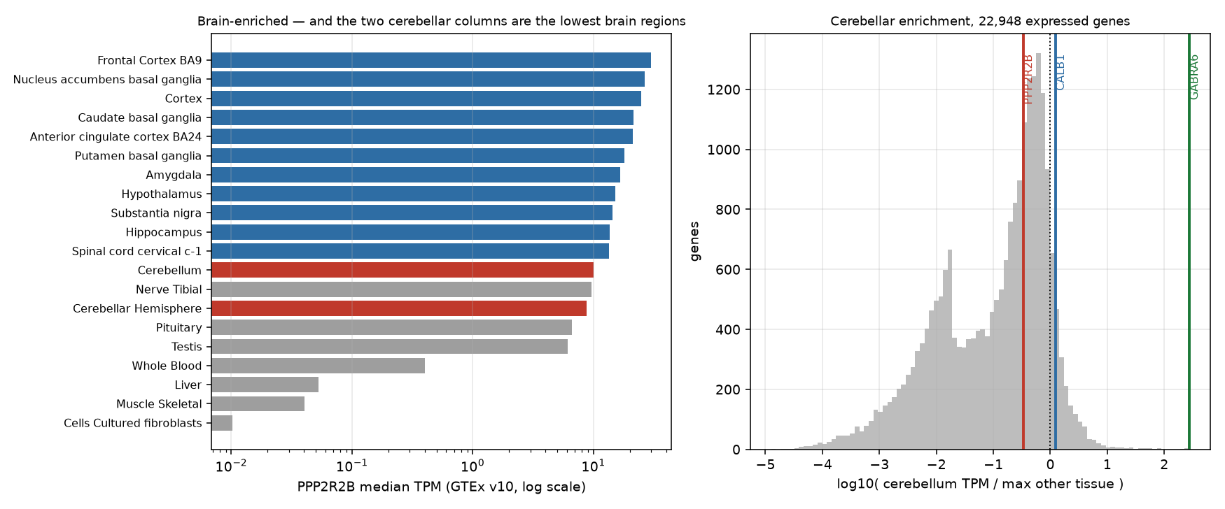
GABRA6 — the granule-cell GABAA receptor subunit — is the single most cerebellum-enriched of the 22,948 genes scored here, at 275× — rank 1 by this score. PPP2R2B sits at 0.34×, rank 8,947 of 22,948 — modestly above the median expressed gene (0.194), and still far below 1, which is what matters: the cerebellum carries a third of what this gene's best other tissue does. Its own paralogue PPP2R2A, which causes no , scores essentially the same.
Three things to hold simultaneously:
- Brain-enrichment is real and large. A ~19-fold margin over median tissue is not noise, and it explains why PPP2R2B disease is neurological rather than systemic.
- Cerebellum-enrichment is absent. Not weak — absent, at the level of the whole tissue.
- Therefore the cerebellar phenotype is a selective-vulnerability problem, not an expression problem. D1 sets out why a cell can die from a gene it expresses no more than its neighbours do; this measurement is what forces you into that chapter rather than letting you off with "the gene is a cerebellar gene".
The statistics here. Every number in this section is a median, and medians do not behave like means. GTEx's median TPM is the middle value across donors for that tissue — a robust location estimate, deliberately insensitive to the one donor with a spectacular outlier, and therefore not an estimate you can add, average or subtract (S3 §2 on estimators and what each one is resistant to). §3 shows the arithmetic consequence directly. The file also publishes no spread at all — no interquartile range, no n per tissue — so a two-fold difference between two tissue medians here comes with no attached uncertainty, and treating it as a tested difference is a category error (S4 §3). What justifies the conclusion above is not one comparison but the shape of the whole ranking: 13 brain regions in a consistent order with the cerebellum at the bottom, and a 22,948-gene reference distribution that puts PPP2R2B in the middle of it.
The confound you have just walked into. A bulk tissue value is a mixture — the weighted average of every cell type in the punch, weighted by how much RNA each contributes (Ch 48 §1 works the arithmetic and shows that two completely different mechanisms give the same bulk number). The cerebellum is the worst possible tissue for this: its neuron count is dominated by granule cells to a degree no other brain region approaches, so the standard expectation is that a bulk cerebellar TPM is close to a granule-cell TPM with everything else diluted into it. A gene expressed strongly and only in would be invisible in this file. What §2 rules out is cerebellum-level enrichment; it cannot rule out cell-type-level enrichment, and the formal name for the correction is (Ch 47 §7) — which §4 sidesteps by measuring the cell types directly, and while doing so overturns the standard expectation for this particular gene.
3. Transcript level: which isoform carries the repeat?
D4 makes a point about the locus that this section turns into a measurement: has many alternative first exons (Ch 06 §9), and the repeat's — , 5′ UTR, or nothing to do with this transcript at all — depends on which transcript you ask about. Hypothesis A needs the repeat to sit in the transcript that actually dominates the . Go and check.
There is no median-transcript flat file in the v10 bucket, and the full transcript matrix is 4.34 GB, so the laptop route is the GTEx portal API.
The answer that is wrong because you believed the first page
curl -s "https://gtexportal.org/api/v2/expression/medianTranscriptExpression?gencodeId=ENSG00000156475.19&datasetId=gtex_v10&itemsPerPage=250" -o tx_page0.json
python - <<'PY'
import json, pandas as pd
d = json.load(open('tx_page0.json'))
print('paging_info:', d['paging_info'])
rows = pd.DataFrame(d['data'])
cb = rows[rows.tissueSiteDetailId == 'Brain_Cerebellum'].sort_values('median', ascending=False)
print('cerebellum rows returned:', len(cb))
print(cb[['transcriptId','median']].head(3).to_string(index=False))
PY
paging_info: {'numberOfPages': 5, 'page': 0, 'maxItemsPerPage': 250, 'totalNumberOfItems': 1134}
cerebellum rows returned: 19
transcriptId median
ENST00000504198.5 6.26
ENST00000394413.7 2.97
ENST00000394411.9 2.38That looks like a complete answer and is not one. 21 transcripts × 54 tissues = 1,134 rows, and the API returned 250. It told you so, in paging_info, in a field it is very easy to discard while reaching for ['data']. Tissues come back in alphabetical order, so page 0 ends partway through Brain_Cerebellum — 19 of the 21 transcripts, cut off mid-tissue. Fetch all five pages:
python - <<'PY'
import json, urllib.request, pandas as pd
rows = []
for p in range(5):
    u = ("https://gtexportal.org/api/v2/expression/medianTranscriptExpression"
         f"?gencodeId=ENSG00000156475.19&datasetId=gtex_v10&itemsPerPage=250&page={p}")
    rows += json.load(urllib.request.urlopen(u))['data']
d = pd.DataFrame(rows)
d.to_csv('ppp2r2b_tx_medians.tsv', sep='\t', index=False)
print('rows', len(d), ' transcripts', d.transcriptId.nunique(), ' tissues', d.tissueSiteDetailId.nunique())
assert len(d) == d.transcriptId.nunique() * d.tissueSiteDetailId.nunique()   # the check page 0 fails

cb = d[d.tissueSiteDetailId == 'Brain_Cerebellum'].sort_values('median', ascending=False)
print(cb[['transcriptId','median']].head(4).to_string(index=False))

page0 = {r['transcriptId'] for r in json.load(open('tx_page0.json'))['data']
         if r['tissueSiteDetailId'] == 'Brain_Cerebellum'}
print('\nmissing from page 0:', sorted(set(cb.transcriptId) - page0))
PY
rows 1134 transcripts 21 tissues 54
transcriptId median
ENST00000530902.5 9.03
ENST00000504198.5 6.26
ENST00000394413.7 2.97
ENST00000394411.9 2.38
missing from page 0: ['ENST00000530902.5', 'ENST00000532154.5']The transcript truncated off page 0 was the most abundant one in the cerebellum. Silent truncation does not corrupt data randomly; it corrupts it in whatever order the server happened to use, and here that put the top answer just past the cut. This is the same class of error as lab-06's replicate trap: nothing fails, nothing warns, and the conclusion is wrong.
Where does each transcript start, relative to the repeat?
Now join the abundances to structure. The repeat, per lab-11, is chr5:146,878,728–146,878,759 (GRCh38) in 1-based inclusive coordinates (STRchive's interval; the ExpansionHunter catalog's is 2 bp shorter — hold that thought). PPP2R2B is on the minus strand, so a transcript's start site is its higher coordinate.
curl -s -H "Content-Type:application/json" \
  "https://rest.ensembl.org/lookup/id/ENSG00000156475?expand=1" -o ppp2r2b_ensembl.json
python - <<'PY'
import json, pandas as pd
g = json.load(open('ppp2r2b_ensembl.json'))
REP = (146878728, 146878759)                      # 1-based inclusive, GRCh38
print('gene', g['seq_region_name'], g['start'], '-', g['end'], 'strand', g['strand'],
      '  transcripts in current Ensembl:', len(g['Transcript']))
tx  = pd.read_csv('ppp2r2b_tx_medians.tsv', sep='\t')
piv = tx.pivot_table(index='transcriptId', columns='tissueSiteDetailId', values='median')

def describe(t):
    exons = sorted(t['Exon'], key=lambda e: -e['end'])      # minus strand: exon 1 is highest
    e1 = exons[0]
    overlap  = max(0, min(e1['end'], REP[1]) - max(e1['start'], REP[0]) + 1)
    intronic = all(e['end'] < REP[0] or e['start'] > REP[1] for e in exons) and t['end'] > REP[1]
    return t['end'], t['end'] - REP[1], overlap, ('intronic' if intronic else '-')

info = {t['id']: describe(t) for t in g['Transcript']}
rows = []
for tid in piv.index:
    if tid.split('.')[0] not in info: continue
    tss, dist, ov, note = info[tid.split('.')[0]]
    rows.append((tid, round(piv.loc[tid, 'Brain_Cerebellum'], 2),
                 round(piv.loc[tid, 'Brain_Frontal_Cortex_BA9'], 2), tss, dist, ov, note))
df = pd.DataFrame(rows, columns=['transcript', 'cerebellum_TPM', 'frontalBA9_TPM',
                                 'TSS', 'TSS_minus_repeat_end', 'exon1_overlap_bp', 'repeat_is'])
print(df.sort_values('cerebellum_TPM', ascending=False).head(8).to_string(index=False))

carry = df[df.exon1_overlap_bp > 0]
for tissue, col in [('cerebellar', 'cerebellum_TPM'), ('frontal-cortex', 'frontalBA9_TPM')]:
    print('\nrepeat-bearing exon 1: %.2f of %.2f %s TPM (%.0f%%)'
          % (carry[col].sum(), df[col].sum(), tissue, 100*carry[col].sum()/df[col].sum()))
print('\nsum of transcript medians, cerebellum: %.2f — gene-level median from section 2: 10.02'
      % df.cerebellum_TPM.sum())
PY
gene 5 146580742 - 147084784 strand -1 transcripts in current Ensembl: 37
transcript cerebellum_TPM frontalBA9_TPM TSS TSS_minus_repeat_end exon1_overlap_bp repeat_is
ENST00000530902.5 9.03 33.90 146878894 135 32 -
ENST00000504198.5 6.26 8.70 147081543 202784 0 intronic
ENST00000394413.7 2.97 3.66 147081429 202670 0 intronic
ENST00000394411.9 2.38 5.42 146878757 -2 30 -
ENST00000453001.5 0.93 3.96 146878785 26 32 -
ENST00000336640.10 0.89 16.16 147055974 177215 0 intronic
ENST00000504565.1 0.49 0.63 147081293 202534 0 intronic
ENST00000508267.5 0.36 0.60 147081470 202711 0 intronic
repeat-bearing exon 1: 12.34 of 23.53 cerebellar TPM (52%)
repeat-bearing exon 1: 43.28 of 77.47 frontal-cortex TPM (56%)
sum of transcript medians, cerebellum: 23.53 — gene-level median from section 2: 10.02This is the locus anatomy of D4, derived rather than asserted. Four distinct relationships between one repeat and one gene:
| Transcript | TSS (GRCh38) | Repeat's position in it | Cerebellum TPM |
|---|---|---|---|
| ENST00000530902.5 | 146,878,894 | entirely inside exon 1, 135 bp downstream of the TSS — 5′ UTR | 9.03 |
| ENST00000453001.5 | 146,878,785 | entirely inside exon 1, 26 bp downstream of the TSS — 5′ UTR | 0.93 |
| ENST00000394411.9 | 146,878,757 | straddles the TSS — 30 bp transcribed, 2 bp upstream | 2.38 |
| ENST00000504198.5 | 147,081,543 | 203 kb away, deep in 2 | 6.26 |
The 1999 report placed the tract 133 nt upstream of the then-known start site, i.e. in the promoter; later work moved it into the 5′ UTR. Both readings are correct, about different transcripts, and you can now see exactly why: transcripts starting a few hundred bases apart put the same 32 bp in the promoter, in the 5′ UTR, or in an intron (Ch 22 §2 on why those are different regulatory parts). Sharper still — for ENST00000394411.9 the classification depends on two base pairs of locus definition. Under STRchive's 32 bp interval the repeat overlaps that transcript's first exon by 30 bp with 2 bp upstream; under the ExpansionHunter catalog's 30 bp interval the repeat lies entirely within the first exon. Two authoritative databases, one locus, and an annotation that flips on the boundary convention.
One thing this table deliberately does not do: attach the literature's isoform names to these accessions. The papers argue in terms of Bβ1 and Bβ2, and of first-exon variants labelled 7B7D and 7C7D in the original PPP2R2B exon numbering (D4). No database column carries that mapping, and guessing which ENST is "Bβ1" from abundance and rough position is exactly the kind of inference that turns into a citation. If you need the mapping, derive it — pull the exon structures and the protein N-termini and match them against the figures in the primary papers — and if you cannot, say the accessions and stop. A transcript identifier is not an isoform name, and the between them is work.
Three further readings, none of which help Hypothesis A:
The repeat-bearing transcripts are about half the gene's output — in both tissues. 52% in cerebellum, 56% in frontal cortex. If the repeat's effect ran through a cerebellum-specific preference for the repeat-bearing first exon, that ratio would differ. It does not.
The most abundant repeat-bearing transcript is 3.8× higher in frontal cortex than in cerebellum (33.90 against 9.03). Descending from gene level to transcript level did not recover cerebellar specificity; it made the cortical bias larger.
The medians do not add up, and should not. Transcript medians sum to 23.53 in the cerebellum while the gene median is 10.02. That is not an inconsistency in GTEx: the median of a sum is not the sum of medians, and each transcript's median is taken over donors independently, so different donors supply the middle value in different rows. Never sum a column of published medians and compare it to a published total (S3 §2). The percentages above survive only because numerator and denominator are computed the same wrong way and the bias largely cancels — which is a reason to quote them to the nearest whole percent and no finer.
Why isoform-level numbers deserve less trust than gene-level ones. Every transcript TPM above is the output of an expectation-maximisation step that distributed short fragments among 21 candidate isoforms sharing most of their sequence — the same EM you ran in lab-06 §4, at far worse odds. Reconstructing full-length isoforms from short fragments is genuinely underdetermined: the data do not contain the answer, and the estimate is the model's best guess given a prior (Ch 47 §7). Three consequences bite here. Isoforms differing only in a first exon are the hardest case, because only fragments landing on the distinguishing exon carry any information and every other read is uninformative between them — and that is precisely the distinction this section rests on. Annotation moves the answer: RefSeq lists 10 transcript variants for this gene, GTEx v10 quantified 21, the current Ensembl release models 37, so you are not measuring the gene, you are measuring the gene as annotated by one release. And the distinguishing exon is the one containing a trinucleotide repeat — low-complexity sequence, where both alignment and are at their least trustworthy. Long reads sequence whole molecules and largely dissolve the problem (Ch 40 §3) — the same argument lab-11 makes about sizing the repeat itself.
4. Cell types: who inside the cerebellum transcribes it? ★★
§2 could not distinguish "the gene is uniformly modest across cerebellar cells" from "the gene is concentrated in and diluted by granule cells". This is the question that decides whether Hypothesis A survives at cell-type resolution, and it needs single nuclei.
The Human Brain Cell Atlas (Siletti et al. 2023) publishes each dissection as a downloadable .h5ad. Take the cerebellar vermis: 71,874 nuclei, 431 MB, no registration.
curl -sL -O https://datasets.cellxgene.cziscience.com/d8c637a7-1dba-40e1-90f2-ddfdbe03fd3b.h5ad
mv d8c637a7-1dba-40e1-90f2-ddfdbe03fd3b.h5ad cerebellar_vermis.h5ad
python - <<'PY'
import scanpy as sc, time, resource
t0 = time.time(); a = sc.read_h5ad('cerebellar_vermis.h5ad')
print('load %.1f s  shape %s  peak RSS %.2f GB'
      % (time.time()-t0, a.shape, resource.getrusage(resource.RUSAGE_SELF).ru_maxrss/1e9))
print(a.uns['title'])
print(a.obs['cell_type'].value_counts().head(8).to_string())
print('Purkinje cells:', int((a.obs.cell_type == 'Purkinje cell').sum()))
PY
load 3.6 s shape (71874, 58232) peak RSS 2.63 GB
Dissection: Cerebellum (CB) - Cerebellar Vermis - CBV
cell_type
cerebellar granule cell 44334
cerebellar inhibitory GABAergic interneuron 9616
Bergmann glial cell 6614
oligodendrocyte 4357
oligodendrocyte precursor cell 3862
microglial cell 1373
unipolar brush cell 716
endothelial cell 278
Purkinje cells: 10Stop at that last line before doing anything quantitative. Ten Purkinje cells out of 71,874. The cell type destroys — the cell type this entire lab exists to ask about — is 0.014% of the atlas. The last subsection of §4 is about why, and what it costs you.
Expression per cell type
The matrix X holds raw nuclear counts (integer row sums, no raw slot, no layers), so normalise before comparing anything. Pseudobulk is the right summary here: pool each cell type's counts and divide by that type's pooled depth, which weights cells by information rather than letting a shallow nucleus vote as loudly as a deep one.
python - <<'PY'
import scanpy as sc, numpy as np, pandas as pd
a   = sc.read_h5ad('cerebellar_vermis.h5ad')
n2i = pd.Series(a.var_names.values, index=a.var['feature_name'].astype(str).values)
col = lambda sym: np.asarray(a[:, n2i[sym]].X.todense()).ravel().astype('float64')
df  = pd.DataFrame({'ct'     : a.obs['cell_type'].astype(str).values,
                    'depth'  : np.asarray(a.X.sum(1)).ravel().astype('float64'),
                    'PPP2R2B': col('PPP2R2B'),
                    'CALB1'  : col('CALB1'),        # Purkinje marker
                    'GABRA6' : col('GABRA6')})      # granule marker
g     = df.groupby('ct')
cp10k = lambda sym: g.apply(lambda d: 1e4 * d[sym].sum() / d.depth.sum(), include_groups=False)
t = pd.DataFrame({'n'           : g.size(),
                  'median_UMI'  : g['depth'].median(),
                  'pct_detected': g['PPP2R2B'].apply(lambda s: 100 * (s > 0).mean()),
                  'PPP2R2B'     : cp10k('PPP2R2B'),
                  'CALB1'       : cp10k('CALB1'),
                  'GABRA6'      : cp10k('GABRA6')})
t['share_of_PPP2R2B'] = 100 * g['PPP2R2B'].sum() / df.PPP2R2B.sum()
print(t[t.n >= 100].sort_values('PPP2R2B', ascending=False).round(2).to_string())
print('\nPurkinje row (n = 10):')
print(t.loc[['Purkinje cell']].round(2).to_string())
print('\nwhole-dissection pseudobulk PPP2R2B: %.2f per 10,000 UMIs'
      % (1e4 * df.PPP2R2B.sum() / df.depth.sum()))
PY
n median_UMI pct_detected PPP2R2B CALB1 GABRA6 share_of_PPP2R2B
ct
Bergmann glial cell 6614 5126.0 99.91 43.65 0.09 0.05 50.84
oligodendrocyte 4357 4155.0 99.54 41.63 0.02 0.05 28.25
astrocyte 203 3446.0 97.54 26.66 0.00 0.07 0.70
oligodendrocyte precursor cell 3862 5198.5 95.60 12.00 0.02 0.05 8.19
unipolar brush cell 716 13428.5 65.36 1.74 0.02 0.08 0.56
cerebellar granule cell 44334 3964.5 31.69 1.29 0.02 2.61 8.43
cerebellar inhibitory GABAergic interneuron 9616 11895.5 32.08 0.64 0.09 0.75 2.43
fibroblast 173 3104.0 8.09 0.52 0.07 0.05 0.01
microglial cell 1373 2332.0 4.37 0.18 0.03 0.07 0.02
pericyte 176 2924.5 5.11 0.16 0.00 0.05 0.00
endothelial cell 278 3040.5 3.96 0.15 0.03 0.06 0.00
Purkinje row (n = 10):
n median_UMI pct_detected PPP2R2B CALB1 GABRA6 share_of_PPP2R2B
ct
Purkinje cell 10 59477.0 80.0 5.8 7.44 0.22 0.11
whole-dissection pseudobulk PPP2R2B: 7.46 per 10,000 UMIsPlot it beside the cell census that produced it — a bar chart of cell-type means without the counts is the single most misleading figure in single-cell work:
python - <<'PY'
import scanpy as sc, numpy as np, pandas as pd, matplotlib
matplotlib.use('Agg'); import matplotlib.pyplot as plt
a   = sc.read_h5ad('cerebellar_vermis.h5ad')
n2i = pd.Series(a.var_names.values, index=a.var['feature_name'].astype(str).values)
df  = pd.DataFrame({'ct'     : a.obs['cell_type'].astype(str).values,
                    'depth'  : np.asarray(a.X.sum(1)).ravel().astype('float64'),
                    'PPP2R2B': np.asarray(a[:, n2i['PPP2R2B']].X.todense()).ravel().astype('float64')})
g = df.groupby('ct')
t = pd.DataFrame({'n': g.size(),
                  'cp10k': g.apply(lambda d: 1e4*d.PPP2R2B.sum()/d.depth.sum(), include_groups=False)})
t = t[t.n >= 10].sort_values('cp10k')
hot = ('Purkinje cell', 'cerebellar granule cell')

fig, ax = plt.subplots(1, 2, figsize=(12.8, 5.4))
bars = ax[0].barh(range(len(t)), t.cp10k,
                  color=['#c0392b' if i in hot else '#2e6da4' for i in t.index])
for i, (idx, r) in enumerate(t.iterrows()):
    if r.n < 100:                                  # too few nuclei to interpret
        bars[i].set_hatch('///'); bars[i].set_edgecolor('white')
    ax[0].text(r.cp10k + 1, i, f'n={int(r.n):,}', va='center', fontsize=7, color='#444444')
ax[0].set_yticks(range(len(t))); ax[0].set_yticklabels(t.index, fontsize=8)
ax[0].set_xlim(0, 78); ax[0].grid(axis='x', alpha=.3)
ax[0].set_xlabel('PPP2R2B, pseudobulk counts per 10,000 UMIs')
ax[0].set_title('Cerebellar vermis snRNA-seq: glia carry the signal\n'
                '(hatched = fewer than 100 nuclei, read with caution)', fontsize=9)

n = df.groupby('ct').size().sort_values(); n = n[n >= 10]
ax[1].barh(range(len(n)), n.values,
           color=['#c0392b' if i in hot else '#9e9e9e' for i in n.index])
ax[1].set_yticks(range(len(n))); ax[1].set_yticklabels(n.index, fontsize=8)
ax[1].set_xscale('log'); ax[1].grid(axis='x', alpha=.3)
ax[1].set_xlabel('nuclei recovered (log scale)')
ax[1].set_title('71,874 nuclei — and 10 of them are Purkinje cells', fontsize=9)
plt.tight_layout(); plt.savefig('sca12_cerebellum_celltypes.png', dpi=140)
PY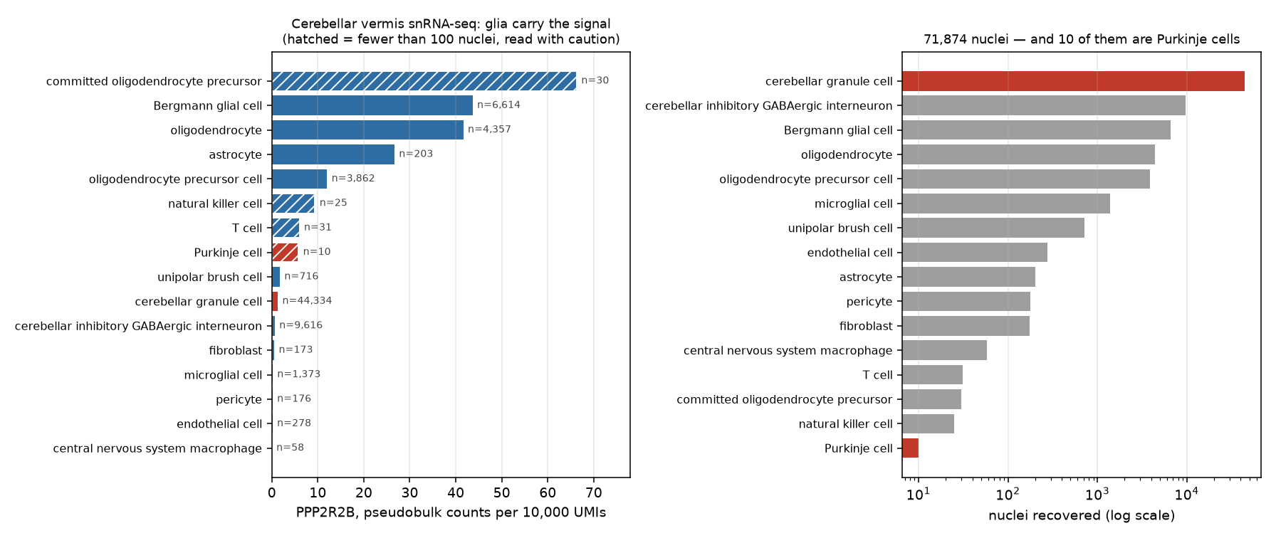
The marker columns confirm the labels before you believe anything else: CALB1 at 7.44 in Purkinje cells and ≈0 everywhere else, GABRA6 highest in granule cells. The is doing what it says.
Now the result, and it is not the result anyone expects:
In this dissection is a glial transcript. Bergmann glia (43.65) and oligodendrocytes (41.63) carry more than 30× the granule-cell level (1.29), and between them supply 79% of every PPP2R2B UMI in the tissue while making up 15% of the nuclei. Granule cells, 62% of the nuclei, supply 8%.
The bulk-dilution story from §2 was right in form and wrong in detail. The standard caution is that bulk is a granule-cell measurement. In nuclear RNA, at least, it is not: the signal for this gene is a Bergmann-glia-and-oligodendrocyte signal with granule cells diluting it downward. Carrying that to a bulk whole-tissue needs one more ingredient — a per-cell-type total-RNA weight — which snRNA-seq cannot supply, because it discards the cytoplasm, and the discarded compartment is largest in exactly the neurons under suspicion here. Which cell type dominates a bulk value is per-gene, set by the product of abundance and per-cell expression, and cannot be read off the tissue's cell census alone.
Purkinje cells are not the answer either. At 5.80 they sit above granule cells and well below the glia — from ten nuclei, which is the next subsection.
Replicate it in the other dissection
One dissection, three donors, one atlas. Before you say any of this out loud, run it again on the lateral hemisphere file (164 MB, 28,028 nuclei):
curl -sL -O https://datasets.cellxgene.cziscience.com/8e5b2509-5b4c-4a9e-895e-b3749849ae1a.h5ad
mv 8e5b2509-5b4c-4a9e-895e-b3749849ae1a.h5ad lateral_hemisphere.h5ad
python - <<'PY'
import scanpy as sc, numpy as np, pandas as pd
a   = sc.read_h5ad('lateral_hemisphere.h5ad')
n2i = pd.Series(a.var_names.values, index=a.var['feature_name'].astype(str).values)
df  = pd.DataFrame({'ct'     : a.obs['cell_type'].astype(str).values,
                    'depth'  : np.asarray(a.X.sum(1)).ravel().astype('float64'),
                    'PPP2R2B': np.asarray(a[:, n2i['PPP2R2B']].X.todense()).ravel().astype('float64')})
g = df.groupby('ct')
t = pd.DataFrame({'n': g.size(),
                  'PPP2R2B': g.apply(lambda d: 1e4*d.PPP2R2B.sum()/d.depth.sum(), include_groups=False)})
print(a.uns['title'], ' ', a.shape)
print(t[t.n >= 50].sort_values('PPP2R2B', ascending=False).round(2).to_string())
print('\nPurkinje cells recovered:', int(t.loc['Purkinje cell','n']),
      ' pseudobulk %.2f' % t.loc['Purkinje cell','PPP2R2B'])
PY
Dissection: Cerebellum (CB) - Lateral hemisphere of cerebellum - CBL (28028, 58232)
n PPP2R2B
ct
oligodendrocyte 1103 50.13
Bergmann glial cell 1070 44.86
astrocyte 108 27.61
oligodendrocyte precursor cell 564 11.66
cerebellar granule cell 23783 1.30
unipolar brush cell 53 1.03
cerebellar inhibitory GABAergic interneuron 960 0.88
fibroblast 69 0.38
microglial cell 218 0.15
Purkinje cells recovered: 1 pseudobulk 4.06The ordering reproduces — Bergmann glia and oligodendrocytes at the top and an order of magnitude clear of everything neuronal, granule cells near the bottom — with the top two swapped and the granule-cell value landing within 1% of the vermis figure (1.30 against 1.29). Two dissections, independently prepared, agreeing to two significant figures on the number that matters. And the second dissection recovered one Purkinje cell.
Ten nuclei, and what they can support
Two Purkinje-cell numbers are now on the table, and they carry very different weight.
The cell count is a solid finding. 10 of 71,874 and 1 of 28,028 is not a fluke of one prep; it is what dissociation does to Purkinje cells. They are the largest neurons in the cerebellar cortex, with dendritic arbours orders of magnitude beyond a granule cell's (D1), they are outnumbered by granule cells by three to four orders of magnitude to begin with, and their nuclei survive tissue dissociation poorly. Every step of the protocol is against them. Note the corroborating signature in the table: the ten recovered nuclei have a median depth of 59,477 UMIs, 15× the granule-cell median — these are enormous nuclei, and the few that survived are exactly the ones a QC threshold on library size would keep (Ch 48 §5 on the cell type a threshold silently deletes).
The expression value is not a solid finding. 5.80 per 10,000 UMIs is a pseudobulk over ten nuclei from a three-donor dissection, and it is dominated by whichever two or three nuclei happened to be deepest. You should not report it as "Purkinje cells express PPP2R2B at a third the Bergmann level"; you should report it as "the ten Purkinje nuclei recovered here are not obviously the high-expressing population, and ten nuclei cannot establish that they are not."
The statistics here. Two different estimation problems sit in this table and only one of them is well-behaved.
pct_detectedis a proportion, and the standard error of a proportion from n observations is √(p(1−p)/n) (S3 §3 on standard error, and S3 §4 on the sampling distribution it is the width of) — at n = 10 and p = 0.8 that is 0.13, so "80% detected" carries an interval spanning roughly half to essentially all, and 8 of 10 versus 10 of 10 is not a distinguishable difference. The pseudobulk value is worse behaved than that, because it is a ratio of two sums across cells with 15-fold different depths: it is not an average of ten equally-weighted observations, it is closer to an average of two or three. The honest move is not to attach a confidence interval to it but to refuse the comparison: a design with 10 cells in one arm and 6,614 in another has no power to detect anything short of an enormous difference (S4 §5 — compute the power of the test you just ran before reporting its null), so a null result here is a failure to measure, not a measurement of no difference. Report the n next to every cell-type mean, always. A bar chart without cell counts hides exactly this.
If 431 MB will not fit. Every CELLxGENE dataset has a zero-install browser Explorer that colours the by any gene and shows expression by cell type. Open the Human Brain Cell Atlas collection, pick the cerebellar dissection, search PPP2R2B, and read the same qualitative ordering off the — glia high, granule cells low, Purkinje cells a handful of dots. Do the quantitative work in §2 and §3, which alone carry the lab's argument. What you lose is the cell counts, which is exactly what the subsection below says matters most, so read the Explorer's per-cluster n before drawing a conclusion from a colour.
5. What this lab can exclude, and what it cannot ★★
Return to §1's table with answers in it. The Grade column uses the ladder D4 defines in its causal-chain section — Established / Supported / Conjectured — so a grading made here carries straight onto D4's arrows and back; the last row needs a fourth state below Conjectured, no evidence either way, for a claim these data do not even argue about from adjacent facts.
| Precondition of Hypothesis A | Verdict from this lab | Grade |
|---|---|---|
| is expressed in | Yes, 10.02 , brain-enriched ~19× over median tissue | Established — bulk medians across 54 tissues, corroborated by the Human Protein Atlas and by Bβ protein detectable only in brain (Strack et al. 1998) |
| It is preferentially expressed there | No. Lowest two of 13 brain regions; enrichment rank 8,947 of 22,948 genes | Established — falsifies the tidy version of the story, and the Human Protein Atlas independently records low regional specificity within brain |
| Cerebellar isoform usage favours the repeat-bearing transcript | No. 52% of cerebellar output against 56% cortical | Supported — short-read isoform estimates, one release |
| The vulnerable cells are the high-expressing cells | Not shown, and not testable here. Glia dominate the signal; 10 Purkinje nuclei recovered | Conjectured — cell-type , not biology |
| The expanded raises PPP2R2B output | Untouched | No evidence either way — the repeat was never genotyped in any of these donors, and none would be expected to carry an expansion |
That last row is the one that matters, and it is worth being blunt about why. Every donor in GTEx v10 and in the Siletti atlas is, for purposes, a control. These files record what PPP2R2B does with two normal-range alleles. Hypothesis A is a claim about what an expanded allele does — STRchive's pathogenic band is 51–78 repeats, but the floor is disputed, with symptomatic patients reported at 40 and 42 and a proposed threshold of ≥43 (D4). No amount of resolution on control tissue — not transcript level, not single nucleus, not spatial — measures the effect of an allele that is not present in the sample. The measurement you have made is of the stage, not the event.
Two failure modes follow from forgetting that, and both appear in the SCA12 literature:
Treating absence of cerebellar enrichment as evidence against SCA12 being a PPP2R2B disease. It is not. The genetic evidence — the , the , the threshold — is independent of expression, and D1 exists because ubiquitously expressed genes routinely kill specific neurons. HTT is expressed everywhere and Huntington disease destroys the striatum. What §2 refutes is a shortcut explanation, not the gene assignment.
Treating expression in controls as a proxy for expression in patients. The direction of the change in patients is exactly what the field disagrees about (D4 tabulates the contradiction: one group reports Bβ1 up, another reports most PPP2R2B isoforms down in patient-derived mature neurons). Nothing in this lab adjudicates that, and a control-tissue atlas cannot.
What would actually settle it
Three designs, in increasing order of what they would prove:
- A repeat-length . the PPP2R2B CAG tract and quantify PPP2R2B expression in the same individuals, then regress expression on repeat length — the molecular-trait regression of Ch 47 §7 and Ch 52, with repeat length in place of a SNP dosage. The open-access files this lab used carry expression and no genotype at all, so the join cannot be made here; it requires the controlled-access layer. Even done well this measures normal-range variation, and extrapolating a slope fitted over 4–31 repeats out to 60 is exactly the kind of extrapolation the course keeps warning about.
- Allele-specific expression in a heterozygous patient. One patient carries a normal and an expanded allele in every cell, sharing a nucleus and a trans environment. Counting reads from each allele at a heterozygous site in the transcript isolates the cis effect with a perfect internal control (Ch 47 §7). The catch is severe and specific to repeats: . Reads from the expanded allele align worse near a tract that is not in the reference, so the expanded allele is systematically under-counted — biased in precisely the direction that would manufacture the "expansion silences the gene" result. Long reads, or a personalised reference, are not optional here.
- Single-nucleus of SCA12 post-mortem cerebellum, with matched controls, and enough Purkinje nuclei to count. This is the experiment. It is also the one this lab has just shown to be hard for a reason that has nothing to do with rarity of the disease: §4 recovered 11 Purkinje nuclei from 99,902 across two dissections of healthy cerebellum. A study powered to compare Purkinje-cell expression between patients and controls needs a protocol that recovers them — nuclear sorting, size-tolerant dissociation, or a spatial assay that never dissociates the tissue at all (Ch 48 §13). And SCA12 post-mortem material is measured in single brains (D5), which sets the ceiling on how soon anyone runs it.
Write three sentences before you close the file. One: what this lab's data can exclude. Two: what it cannot touch. Three: the experiment that would.
A defensible set — compare yours against it rather than copying it. Open control expression data exclude the explanation that SCA12 is cerebellar because PPP2R2B is a cerebellar gene: at tissue level the two cerebellar columns are the lowest of thirteen brain regions and the gene's cerebellar enrichment scores below 1, near the middle of the distribution of 22,948 expressed genes, and at transcript level the cerebellum shows no preference for the repeat-bearing first exon. They cannot say anything about the expanded allele, because no expanded allele exists in any donor here, and they cannot resolve the , because two cerebellar dissections yielded eleven Purkinje nuclei between them. Settling it requires expression measured in carriers with their repeat lengths known in the same individuals — a repeat-length eQTL, or allele-specific expression within single heterozygous patients using reads long enough to escape reference bias at the tract.
Troubleshooting
| Symptom | Cause and fix |
|---|---|
ParserError: Expected 2 fields in line 3 | GCT preamble. skiprows=2 |
| Gene lookup returns an empty frame, no error | GENCODE version suffix: the file stores ENSG00000156475.19. Match on prefix or on the Description symbol column, and assert the result is non-empty |
| Your tissue count is 68, not 54 | The 14 laser-capture sub-columns are still in. Drop them before any cross-tissue median or maximum, or organs with sub-columns get extra votes |
KeyError: 'PPP2R2B' from the h5ad | CELLxGENE .h5ad files index var by Ensembl ID. Build the symbol → ID map from a.var['feature_name'] rather than hard-coding an ID from memory |
| A transcript you expected is missing from the API result | Pagination. paging_info reports numberOfPages; loop until you have totalNumberOfItems rows and assert the count |
| Cell-type means look implausible for rare types | Check n per type in the same table. Anything under ~50 nuclei is a label, not a measurement |
| The h5ad download 404s | Content-addressed URLs rotate when a dataset is revised. Re-resolve from the collection page rather than retrying the dead link |
MemoryError loading the 431 MB file | Peak RSS here was 2.63 GB. Use the 164 MB lateral-hemisphere file, which reproduces the whole result (§4), or the browser Explorer fallback. The 150 MB cerebellar-inhibitory supercluster file is smaller still but contains only interneurons, so it cannot make the across-cell-type comparison at all |
| Your differ from the ones printed here | Name the GTEx release. These are v10; v8 gives similar but not identical medians, and future releases will move them again |
What you can now do
| Step | What ran | The number that mattered |
|---|---|---|
| §2 | GTEx v10 median- GCT, 8.8 MB | 10.02 TPM, 12th of 13 brain regions; enrichment rank 8,947 / 22,948 |
| §3 | GTEx portal API, 5 pages; Ensembl REST | Repeat-bearing exon 1 = 52% of cerebellar output vs 56% cortical; top transcript missed on page 0 |
| §4 | Siletti atlas, 2 dissections, scanpy | Bergmann glia + oligodendrocytes = 79% of ; 10 Purkinje nuclei of 71,874 |
| §5 | — | Every donor is a control: zero evidence about the expanded |
The transferable lesson is not about . It is that public data answer the question they were collected to answer, and the skill is stating precisely which question that is before the plot seduces you into a different one. GTEx was built to describe normal human tissue expression, and it does that superbly; asked "does the SCA12 expansion raise PPP2R2B?" it returns a beautiful, well-normalised, entirely irrelevant answer.
Check yourself
1. A colleague plots across GTEx, sees at 10 against 0.04 in skeletal muscle, and writes "PPP2R2B is a cerebellar gene, which explains the cerebellar of ". Both numbers are correct. What is wrong with the sentence, and what would a correct version say?
Answer
The comparison is against the wrong reference class. 10 TPM against 0.04 establishes brain-enrichment, which nobody disputes and which explains only why the disease is neurological. The claim being made is about the cerebellum within the brain, and that comparison runs the other way: the cerebellum at 10.02 TPM is 12th of 13 GTEx brain regions, below frontal cortex at 29.71, nucleus accumbens at 26.62 and every other region sampled. The cerebellar hemisphere at 8.78 is 13th.
Scoring the whole transcriptome the same way makes it quantitative. Cerebellum against best non-cerebellar tissue puts GABRA6 at 275× (rank 1 of 22,948 expressed genes) and PPP2R2B at 0.34×, rank 8,947 — near the middle of the distribution, and well below the score of 1 that even parity with one other tissue would require. Its paralogue PPP2R2A, which causes no , scores 0.35×. "Cerebellar gene" has an operational meaning and PPP2R2B does not meet it.
A correct version: "PPP2R2B is strongly brain-enriched but not cerebellum-enriched; the cerebellar phenotype of SCA12 is therefore an instance of selective neuronal vulnerability rather than a consequence of where the gene is transcribed."
The general habit worth taking: whenever a paper says a gene is "enriched" somewhere, ask relative to what, and check the rank rather than a ratio against the tissue where the gene is least expressed. Any brain gene beats fibroblasts.
2. §4 found PPP2R2B highest in Bergmann glia and oligodendrocytes, and low in granule cells. §2's standard caution was that bulk cerebellum is dominated by granule-cell RNA. Reconcile them, and say what the reconciliation implies for reading any bulk value.
Answer
Both are about composition, and they do not contradict each other — the second is a statement about the tissue, the first about one gene in it.
Bulk cerebellum is granule-cell-dominated by nuclei: 44,334 of 71,874 in the vermis dissection, 62%. But a bulk value is the sum of (cells × per-cell expression), not of cells. For PPP2R2B the per-cell term runs the other way — per nucleus (cp10k × median depth / 10⁴), Bergmann glia hold about 22.4 PPP2R2B counts against 0.51 in granule cells, a ≈44-fold gap that overwhelms the abundance advantage. Note that the cp10k values alone (43.65 against 1.29) are compositional fractions, not per-cell abundances; the share_of_PPP2R2B column is computed from raw counts and so carries the depth-weighting correctly. The result: Bergmann glia (9% of nuclei) supply 51% of PPP2R2B and oligodendrocytes (6%) supply 28%, while granule cells (62%) supply 8%.
The implication is the useful part. Which cell type dominates a bulk measurement is a per-gene property, determined by the product of abundance and expression, and cannot be read off a tissue's cell census. "Bulk cerebellum ≈ granule cells" is a decent prior for a gene you know nothing about and a bad assumption for any specific gene. The only way to know is to decompose — against a reference (Ch 47 §7) or direct single-cell measurement (Ch 48).
A second implication for SCA12 specifically: if the dosage-sensitive cells were glia rather than neurons, the mechanism would look quite different. This lab cannot decide that — RNA is not protein, three donors is not a cohort, and one atlas is not a literature — but it is a hypothesis this measurement generated and nobody's expression intuition would have.
3. You have the cell-type table from §4 and want to report " express PPP2R2B at 5.80 per 10,000 UMIs, well below Bergmann glia at 43.65". Why should you not, and what should the sentence say instead?
Answer
Because 5.80 comes from 10 nuclei and 43.65 from 6,614, and the comparison has no power to support either "well below" or its negation.
Three specific problems. The pseudobulk value is a ratio of sums over cells whose depths differ 15-fold — the ten Purkinje nuclei have a median 59,477 UMIs against 3,964 for granule cells — so it is effectively an average over the two or three deepest nuclei, not ten equally-weighted observations. The detection rate that accompanies it, 80%, has a standard error of √(0.8×0.2/10) = 0.13 at that sample size, so it is compatible with anything from about half to all (S3 §3). And a comparison of 10 against 6,614 detects only enormous differences, so failing to see one is a failure to measure, not a measurement of no difference (S4 §5).
What to write instead: "Purkinje cells are essentially absent from these dissections — 10 of 71,874 nuclei in the vermis and 1 of 28,028 in the lateral hemisphere — so this dataset cannot establish their PPP2R2B level. The question of Purkinje-cell enrichment remains open, and answering it requires a protocol that recovers Purkinje nuclei."
The habit: put n beside every group mean, and when n is small enough that the mean is uninterpretable, report the n as the finding. Here the count is genuinely more informative than the expression value — it tells you why this question has not been settled.
4. The §3 API call returned 250 rows and named the cerebellum's top isoform as ENST00000504198.5 at 6.26 TPM. The full result names ENST00000530902.5 at 9.03. Nothing errored. What class of bug is this, and what would you add to a pipeline so it cannot recur?
Answer
Silent truncation: an API that returns a valid, well-formed, incomplete answer and reports the incompleteness in a field you are free to ignore. The response carried paging_info: {'numberOfPages': 5, 'totalNumberOfItems': 1134}, and 21 transcripts × 54 tissues = 1,134 rows, so page 0 held 22% of the data. Tissues come back alphabetically, so the cut landed mid-Brain_Cerebellum, returning 19 of 21 transcripts — and one of the two omitted rows was the highest-expressing transcript in the tissue.
The class is broader than pagination. It is the same failure mode as lab-06's replicate trap and as this lab's own version-suffix join: the operation succeeds, the output is the right shape, and it is wrong. Errors you can see are cheap; results that are quietly partial are what propagate into papers.
The defence is an assertion at every boundary where the data could be truncated:
- After a paginated fetch, assert
len(rows) == paging_info['totalNumberOfItems'], or loop until it holds. Never take['data']from page 0 alone. - After any join or lookup, assert the result is non-empty and has the expected cardinality — this catches the
ENSG00000156475versusENSG00000156475.19failure in the same net. - Where a total is knowable independently, check it. Here, 21 distinct
transcriptIdvalues × 54 distincttissueSiteDetailIdvalues should equal the row count exactly.
A sanity check on the science also catches it: the top isoform in cerebellum should plausibly appear in other tissues too, and a transcript list that varies in length between tissues is a tell that rows are missing rather than that biology differs.