S4 — Hypothesis testing, and what it doesn't tell you
Read before: Ch 12 · Time: ~55 min
All code in this chapter runs from the repository root — the directory holding README.md and .venv — with source .venv/bin/activate, and addresses data as labs/data/….
A variant caller hands you three million sites. Some fraction of them are not real — the reads mismapped, one failed to amplify, two paralogous genes collapsed into one locus. Nobody is going to inspect them by eye. So you need a machine that takes counts and returns a number saying how surprised should I be, if nothing is wrong? That machine is the significance test, and in genomics it is applied at industrial scale: Hardy–Weinberg filtering (Ch 26), variant QC (Ch 46), every locus in a (Ch 51), every gene in an experiment (Ch 47). Every one of those chapters is still ahead of you. They are named as destinations, not prerequisites: nothing below assumes you have read them, and the genetics this chapter needs is defined here as statistics before it is used.
This chapter builds that machine and then spends most of its length on the far more useful question of what the machine does not tell you. That imbalance is deliberate. The mechanics take one section. The misreadings take the rest of your career.
What you'll be able to do
- Name the four components of a significance test and say which one carries the modelling risk
- Compute a χ² goodness-of-fit test from a genetic hypothesis, get the degrees of freedom right — including when a parameter was estimated from the same data — and say where the asymptotic approximation fails and an exact test is required
- State five things a p-value is not, and compute the base-rate calculation that shows why
- Compute the power of a test from effect size, sample size and α, and refuse to interpret a non-significant result without it
- Read a p-value histogram from a genome-wide scan as a diagnostic instrument
- Predict how many false positives a scan of m loci will produce, and recognise the analysis choices that silently multiply m
The core idea
A significance test is proof by contradiction with a probability attached, and it runs in exactly one direction.
You assume something specific and boring — "this population is in Hardy–Weinberg proportions", "this gene is not differentially expressed". That assumption, the null hypothesis, is specific enough to generate data. You then compute a number from your real data, a test statistic, chosen so that big values mean "unlike what the null produces". You work out the distribution that statistic would have if the null were true. And you ask: what fraction of that null distribution is at least as extreme as what I actually saw? That fraction is the p-value.
Small p means: the null makes my data look weird. That is all it means. It says nothing about how likely the null is, nothing about how big the effect is, and — this is the one that repeatedly ruins studies — a large p says nothing at all, because "the null makes my data look unremarkable" is also true of every null that is wrong in a way too small for your sample size to notice.
The p-value is a property of the null hypothesis, not of your hypothesis. It answers "how often would data like mine arise if nothing were going on?" — and never the question you actually care about, which is "given my data, what is going on?" Getting from the first to the second requires a prior, and that is S6.
1. The four moving parts
All of it, on real data. Load the 1000 Genomes chr22 window that ships with the labs — 2,548 people, every biallelic SNV in a 1 Mb region. Note the deliberate choice of file: chr22_qc has already been Hardy–Weinberg-filtered at p < 10⁻⁶, so testing HWE on it would be circular. The raw has not, and it needs no external tools to read.
cd /path/to/learn-genomics   # the directory holding README.md and .venv
source .venv/bin/activate
import gzip, numpy as np, pandas as pd
def load_vcf(path):
"""Biallelic SNVs from a 1000G VCF -> (variants x samples) ALT dosage 0/1/2."""
pos, rows = [], []
with gzip.open(path, "rt") as f:
for line in f:
if line.startswith("##"):
continue
fl = line.rstrip("\n").split("\t")
if line.startswith("#CHROM"):
samples = np.array(fl[9:]); continue
if len(fl[3]) != 1 or len(fl[4]) != 1:
continue # skip indels
pos.append(int(fl[1]))
rows.append([(g[0] == "1") + (g[2] == "1") for g in fl[9:]])
return np.array(pos), np.array(rows, dtype=np.int8), samples
pos, G, samples = load_vcf("labs/data/chr22_sub.vcf.gz")
panel = pd.read_csv("labs/data/panel.txt", sep="\t").set_index("sample").reindex(samples)
print(G.shape, "variants x samples")
print(panel["super_pop"].value_counts().to_dict())(27895, 2548) variants x samples
{'AFR': 660, 'EAS': 504, 'EUR': 503, 'SAS': 489, 'AMR': 347}(The population labels sum to 2,503, not 2,548: panel.txt covers only the unrelated subset, and the remaining 45 samples get NaN, which value_counts drops. Worth noticing — a count that doesn't add up is usually the first sign of a join you got wrong.)
Take the first common SNP, chr22:20,000,722 (G>A), in the 503 European-ancestry samples. The counts are 166 GG, 237 GA, 100 AA.
| Component | Here |
|---|---|
| Null hypothesis | Genotypes are a random pairing of : p², 2pq, q² |
| Test statistic | χ² = Σ (observed − expected)² / expected |
| Null distribution | χ² with 1 degree of freedom |
| p-value | P(statistic ≥ observed) under that distribution |
from scipy import stats

n_GG, n_GA, n_AA = 166, 237, 100
N = n_GG + n_GA + n_AA

p = (2*n_GG + n_GA) / (2*N)          # frequency of G, estimated FROM THESE DATA
q = 1 - p
exp = np.array([p**2, 2*p*q, q**2]) * N
obs = np.array([n_GG, n_GA, n_AA])

X2 = ((obs - exp)**2 / exp).sum()
print(f"N={N}  p(G)={p:.4f}")
print("observed", obs)
print("expected", exp.round(2))
print(f"X2 = {X2:.4f}")
print(f"p-value, df=1 (correct)   = {stats.chi2.sf(X2, 1):.4f}")
print(f"p-value, df=2 (the error) = {stats.chi2.sf(X2, 2):.4f}")

# scipy's one-liner. ddof is SUBTRACTED from k-1, so ddof=1 gives df = 3-1-1 = 1
print(stats.chisquare(obs, exp, ddof=1))
N=503 p(G)=0.5656
observed [166 237 100]
expected [160.92 247.17 94.92]
X2 = 0.8516
p-value, df=1 (correct) = 0.3561
p-value, df=2 (the error) = 0.6533
Power_divergenceResult(statistic=np.float64(0.8515629301279481), pvalue=np.float64(0.3561105681398722))Three parts of that are routine arithmetic. The part that carries all the risk is the expected counts, because they encode the genetic hypothesis. Change the hypothesis and the expectations change; the machinery does not care and will happily return a p-value for a null nobody believes (Ch 12 is the genetics-side treatment of exactly this).
Note scipy.stats.chisquare's ddof: it is subtracted from k − 1, so ddof=1 means df = 1. Leave it at its default of 0 and you silently get df = 2 and the wrong answer.
2. Where the degrees of freedom come from
Three classes, so the intuition says df = 3 − 1 = 2. That is wrong here, and the reason is worth seeing rather than memorising: the p was estimated from the same counts you are testing. The expected values were bent toward the data before the comparison, so the residuals have less room to move than they otherwise would.
The rule is df = (classes) − 1 − (parameters estimated from these data) = 3 − 1 − 1 = 1. You do not have to take that on faith — simulate the null and look:
rng = np.random.default_rng(0)
N, p_true, B = 503, 0.5656, 200_000

# 200,000 populations that really ARE in Hardy-Weinberg
draws = rng.multinomial(N, [p_true**2, 2*p_true*(1-p_true), (1-p_true)**2], size=B)
n0, n1, n2 = draws.T

def X2_from(n0, n1, n2, p):
    e = np.stack([p**2, 2*p*(1-p), (1-p)**2], axis=-1) * N
    o = np.stack([n0, n1, n2], axis=-1)
    return ((o - e)**2 / e).sum(-1)

X2_refit = X2_from(n0, n1, n2, (2*n0 + n1) / (2*N))   # p re-estimated each time
X2_known = X2_from(n0, n1, n2, p_true)                # p handed to us for free

print(f"mean X2, p re-estimated from the data : {X2_refit.mean():.3f}   (df = 1)")
print(f"mean X2, p known in advance           : {X2_known.mean():.3f}   (df = 2)")
print(f"simulated p-value = P(X2 >= 0.8516)   = {(X2_refit >= 0.8516).mean():.4f}")
print(f"analytic  p-value, chi2 df=1          = {stats.chi2.sf(0.8516, 1):.4f}")
print(f"false-positive rate at alpha=0.05, df=1: {(stats.chi2.sf(X2_refit,1) < 0.05).mean():.4f}")
print(f"false-positive rate at alpha=0.05, df=2: {(stats.chi2.sf(X2_refit,2) < 0.05).mean():.4f}")
mean X2, p re-estimated from the data : 1.004 (df = 1)
mean X2, p known in advance : 2.001 (df = 2)
simulated p-value = P(X2 >= 0.8516) = 0.3572
analytic p-value, chi2 df=1 = 0.3561
false-positive rate at alpha=0.05, df=1: 0.0502
false-positive rate at alpha=0.05, df=2: 0.0144The mean of a χ² distribution equals its df, and the simulation reads it straight off: 1.004 when p is fitted, 2.001 when p is given. Estimating one parameter costs exactly one degree of freedom. It also shows two things worth carrying:
- You can always build a null distribution by brute force. Simulate under the null, compute the statistic, count the tail. Every analytic null distribution is a shortcut for this, and when your situation has no textbook null — a weird statistic, a small sample, a bespoke model — the simulation is the test (this is the permutation/parametric-bootstrap idea, used throughout Ch 33).
- The wrong df is not a harmless rounding error. With df = 2 the test rejects 1.4% of the time instead of 5% — it is conservative, which sounds safe and is not: you have thrown away most of your power for nothing, and you will never see the real departures you missed.
3. What a p-value is not
| It is not | Why not |
|---|---|
| P(null is true | data) | It is P(data this extreme | null true). Reversing a conditional requires a prior. P(rain | clouds) ≠ P(clouds | rain) |
| The probability the result is a fluke | Same reversal. The fluke rate depends on how many nulls were true to begin with — see below |
| A measure of effect size | p depends on effect size and sample size. A trivial effect at N = 10⁶ gives p = 10⁻²⁰; a huge effect at N = 10 gives p = 0.3 |
| Evidence for the null when large | A large p is what you get both when the null is true and when your test is too weak to tell. §5 |
| Repeatable | Under a true alternative, the p-value is itself a random variable with a wide distribution. A study at 50% power replicates half the time by construction |
The first two are the same error, and it is quantifiable. Doing the arithmetic needs an effect size, so name one now, because the rest of this chapter runs on it. For the HWE test the effect size is F, the standardised heterozygote deficit: F = 1 − (observed heterozygotes) / (heterozygotes the p², 2pq, q² proportions expect). F = 0 is exact agreement, F > 0 too few heterozygotes, F < 0 too many. Take it as that statistic and nothing more for now — it is a scaled residual, on a scale that does not depend on the . What a nonzero F means biologically is a Part 5 question, and Ch 26 and Ch 28, both still ahead of you, give it its three standard readings: inbreeding, population structure, and assay failure.
Suppose you are HWE-filtering a million variants; suppose 1% of them are genuinely broken by an assay pathology strong enough to induce F = 0.15, and you have N = 2,000 samples. Of the variants you , what fraction are actually broken?
def power(N, F, alpha):
    """Power of the 1-df HWE test: noncentrality lambda = N*F^2."""
    return stats.ncx2.sf(stats.chi2.ppf(1-alpha, 1), 1, N*F**2)

m, prior_bad, N, F_bad = 1_000_000, 0.01, 2000, 0.15
print(f"{'alpha':>10} {'power':>7} {'true pos':>10} {'false pos':>11} {'PPV':>8}")
for a in [0.05, 1e-3, 1e-6, 1e-8]:
    pw = power(N, F_bad, a)
    tp, fp = m*prior_bad*pw, m*(1-prior_bad)*a
    print(f"{a:>10.0e} {pw:>7.3f} {tp:>10,.0f} {fp:>11,.0f} {tp/(tp+fp):>8.3f}")
alpha power true pos false pos PPV
5e-02 1.000 10,000 49,500 0.168
1e-03 1.000 9,997 990 0.910
1e-06 0.965 9,654 1 1.000
1e-08 0.836 8,358 0 1.000At α = 0.05, 83% of the variants you would throw away are fine, even though every one of them "failed at p < 0.05". Nothing about the arithmetic of the test changed; what changed is the base rate. Move the threshold to 10⁻⁶ and the flagged set is essentially pure while still catching 96.5% of the genuinely broken variants. That calculation is the reason Ch 26 §6, when you reach it, will set the HWE filter at p < 10⁻⁶ rather than 0.05, and the reason a genome-wide association threshold is 5 × 10⁻⁸ rather than anything you would use on a single hypothesis.
4. Type I, Type II, and power
Two ways to be wrong, and they trade off against each other.
| Null actually true | Null actually false | |
|---|---|---|
| Reject | Type I error — rate α | Correct — probability 1 − β = power |
| Fail to reject | Correct | Type II error — rate β |
α is chosen by you. β is not: it falls out of the effect size, the sample size, and α. For the HWE test the algebra is unusually clean. Write the three observed counts as their expectations plus a deviation — n₀ − Np̂² = Np̂q̂F̂, n₁ − 2Np̂q̂ = −2Np̂q̂F̂, n₂ − Nq̂² = Np̂q̂F̂, which is just §3's definition of F̂ rearranged — put them into Σ(observed − expected)²/expected, and every p̂ and q̂ cancels: the statistic is exactly N F̂² on 1 df. So the non-centrality parameter is λ = N F², and power is a tail probability of a non-central χ².
That is the one-parameter case of a fact worth carrying whole. Take any goodness-of-fit test over k classes: the null says the class proportions are π₁ … πk, the truth is some other set p₁ … pk (subscripted, to keep them apart from the p). Then the non-centrality is λ = N Σ (pᵢ − πᵢ)²/πᵢ — the same sum the test statistic computes, with true proportions substituted for observed counts, evaluated on the df the null distribution already has. Put the Hardy–Weinberg alternative (p² + Fpq, 2pq(1 − F), q² + Fpq) through it and the frequencies cancel exactly as they did above, returning λ = N F². Reach for the general form whenever the null has more than two free classes — a 9:3:3:1 dihybrid ratio, a 1:2:1 cross — which is how Ch 12, the chapter you read next, computes the power of a cross before running it.
def power_sim(N, F, alpha, B=20000):
    """Simulate B populations with true inbreeding coefficient F, test HWE, count rejections."""
    p = 0.3
    probs = [p*p + F*p*(1-p), 2*p*(1-p)*(1-F), (1-p)**2 + F*p*(1-p)]
    n0, n1, n2 = rng.multinomial(N, probs, size=B).T
    ph = (2*n0 + n1) / (2*N)
    Fh = (n0/N - ph**2) / (ph*(1-ph))
    return (stats.chi2.sf(N*Fh**2, 1) < alpha).mean()

print(f"{'N':>7} {'F':>6} {'alpha':>8} {'simulated':>10} {'analytic':>9}")
for N, F, a in [(100,0.05,0.05), (1000,0.05,0.05), (10000,0.05,0.05),
                (1000,0.10,0.05), (1000,0.20,0.05),
                (1000,0.10,0.001), (1000,0.10,5e-8)]:
    print(f"{N:>7} {F:>6.2f} {a:>8.0e} {power_sim(N,F,a):>10.3f} {power(N,F,a):>9.3f}")
N F alpha simulated analytic
100 0.05 5e-02 0.079 0.079
1000 0.05 5e-02 0.343 0.353
10000 0.05 5e-02 0.999 0.999
1000 0.10 5e-02 0.873 0.885
1000 0.20 5e-02 1.000 1.000
1000 0.10 1e-03 0.441 0.449
1000 0.10 5e-08 0.012 0.011Simulation and formula agree, which is the point of running both. Read the last three rows together: the same study, the same real departure, tested at three different thresholds, has power 0.885, 0.449 and 0.011. Tightening α to control false positives buys that control with power, and the exchange rate is brutal.
import matplotlib.pyplot as plt
fig, ax = plt.subplots(1, 2, figsize=(10, 3.8))
Fg = np.linspace(0.001, 0.30, 300)
for Nv in [100, 500, 2000, 10000]:
    ax[0].plot(Fg, power(Nv, Fg, 0.05), label=f"N = {Nv:,}")
ax[0].set_xlabel("true departure  F"); ax[0].set_ylabel("power"); ax[0].set_title(r"$\alpha = 0.05$")
Ng = np.logspace(1.5, 6, 300)
for a, lab in [(0.05, r"$\alpha=0.05$"), (1e-3, r"$\alpha=10^{-3}$"),
               (1e-6, r"$\alpha=10^{-6}$"), (5e-8, r"$\alpha=5\times10^{-8}$")]:
    ax[1].plot(Ng, power(Ng, 0.05, a), label=lab)
ax[1].set_xscale("log"); ax[1].set_xlabel("sample size N"); ax[1].set_title("F = 0.05 fixed")
for a_ in ax: a_.axhline(0.8, ls=":", c="k", lw=.8); a_.legend(frameon=False, fontsize=8)
fig.tight_layout(); fig.savefig("../../part-S-statistics/S4-power.png", dpi=130)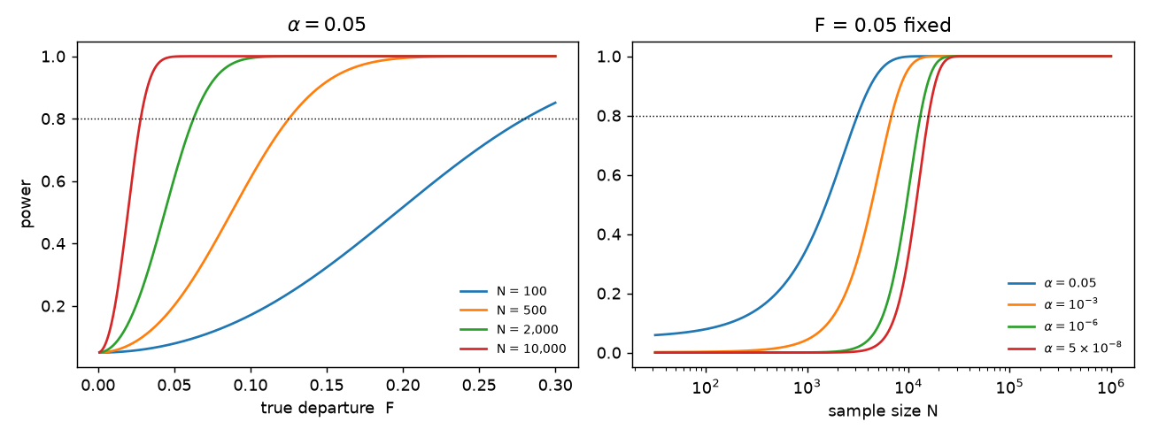
Inverting the relationship gives the design rule. Solving ncx2.sf(crit, 1, λ) = 0.8 for λ:
| α | λ for 80% power | N needed at F = 0.05 | N needed at F = 0.20 |
|---|---|---|---|
| 0.05 | 7.85 | 3,140 | 196 |
| 10⁻³ | 17.07 | 6,830 | 427 |
| 10⁻⁶ | 32.87 | 13,148 | 822 |
| 5 × 10⁻⁸ | 39.60 | 15,840 | 990 |
Sample size scales as 1/effect². Halving the effect you want to detect quadruples the study. This single fact explains the entire trajectory of human genetics from candidate-gene studies of 200 people to biobanks of 500,000 (Ch 51).
5. Absence of evidence: compute the power of the test you just ran
Return to §1: χ² = 0.85, p = 0.36, not significant. It is nearly irresistible to write "the population is in at this locus". Do not. Ask instead what departures that test could have detected. Run it in the 91 British (GBR) samples rather than all 503 Europeans and the question gets sharper:
from scipy.optimize import brentq
for F in [0.05, 0.10, 0.20, 0.25]:
    print(f"  N=91, true F={F:.2f}: power = {power(91, F, 0.05):.3f}")
print(f"  N=91  detects F = {brentq(lambda F: power(91,F,0.05)-0.8, 0.01, 2):.3f} with 80% power")
print(f"  N=503 detects F = {brentq(lambda F: power(503,F,0.05)-0.8, 0.01, 2):.3f}")
N=91, true F=0.05: power = 0.076
N=91, true F=0.10: power = 0.159
N=91, true F=0.20: power = 0.479
N=91, true F=0.25: power = 0.665
N=91 detects F = 0.294 with 80% power
N=503 detects F = 0.125At N = 91 the test rejects 5% of the time when nothing is happening and 7.6% of the time when F = 0.05. It is not measuring anything. To be reliably caught, a departure would have to exceed F ≈ 0.29 — larger than the heterozygote deficit produced by mating full sibs. So the non-significant result excludes essentially nothing of biological interest.
The fix is to report the effect size and its interval instead of the verdict. From χ² = N F̂² on 1 df it follows immediately that √N · F̂ is standard normal under the null, so SE(F̂) ≈ 1/√N and the interval is F̂ ± 1.96/√N. Check it against a bootstrap, which assumes nothing:
g = np.repeat([0, 1, 2], [166, 237, 100])            # the 503 EUR genotypes
def Fhat(g):
    n0, n1, n = (g == 0).sum(), (g == 1).sum(), len(g)
    p = (2*n0 + n1) / (2*n)
    return (n0/n - p*p) / (p*(1-p))

bs = np.array([Fhat(rng.choice(g, len(g), replace=True)) for _ in range(20000)])
print(f"F_hat = {Fhat(g):+.4f}")
print(f"bootstrap SE = {bs.std():.4f}   (1/sqrt(N) = {1/np.sqrt(len(g)):.4f})")
print(f"bootstrap 95% CI = [{np.percentile(bs,2.5):+.3f}, {np.percentile(bs,97.5):+.3f}]")
F_hat = +0.0411
bootstrap SE = 0.0444 (1/sqrt(N) = 0.0446)
bootstrap 95% CI = [-0.047, +0.127]"F̂ = +0.041, 95% CI [−0.048, +0.127]" is a real statement: the data rule out a deficit above about 0.13 and an excess below about −0.05, and are agnostic in between. "p = 0.36, not significant" throws all of that away. A confidence interval contains the test — anything outside it would have been rejected — and adds the one thing the test omits, which is the magnitude. Reach for intervals by default; see S3 for how they are constructed.
6. Running the test for real: HWE across thousands of SNPs
One test tells you little. Thousands of tests tell you about the machinery. If a null is true across a set of loci, the p-values must be uniform on [0,1] — that is what "p-value" means, and it makes the histogram of p-values a diagnostic instrument.
def hwe_scan(Gm, min_maf=0.05):
    """Vectorised HWE chi-square over every variant."""
    N = Gm.shape[1]
    n0 = (Gm == 0).sum(1); n1 = (Gm == 1).sum(1); n2 = (Gm == 2).sum(1)
    p = (2*n0 + n1) / (2*N); q = 1 - p
    keep = np.minimum(p, q) >= min_maf
    F = (n0[keep]/N - p[keep]**2) / (p[keep]*q[keep])
    return F, stats.chi2.sf(N*F**2, 1), keep.sum(), N

for label, mask in [("all 26 populations pooled", np.ones(len(samples), bool)),
                    ("EUR super-population",  (panel["super_pop"] == "EUR").to_numpy()),
                    ("GBR only (British)",    (panel["pop"] == "GBR").to_numpy())]:
    F, pv, m, N = hwe_scan(G[:, mask])
    print(f"{label:26s} N={N:5d}  {m:5d} SNPs   p<0.05: {(pv<0.05).mean():6.1%}   "
          f"p<1e-6: {(pv<1e-6).mean():6.2%}   median F = {np.median(F):+.4f}")
all 26 populations pooled N= 2548 2603 SNPs p<0.05: 64.4% p<1e-6: 31.66% median F = +0.0591
EUR super-population N= 503 2412 SNPs p<0.05: 10.1% p<1e-6: 0.66% median F = +0.0009
GBR only (British) N= 91 2329 SNPs p<0.05: 2.4% p<1e-6: 0.04% median F = +0.0010fig, axs = plt.subplots(1, 3, figsize=(11, 3.2))
for ax, (lab, mask) in zip(axs, [("all 2,548 pooled", np.ones(len(samples), bool)),
("EUR (N=503)", (panel["super_pop"] == "EUR").to_numpy()),
("GBR (N=91)", (panel["pop"] == "GBR").to_numpy())]):
_, pv, _, _ = hwe_scan(G[:, mask])
ax.hist(pv, bins=20, range=(0, 1), color="#4477aa", edgecolor="w")
ax.axhline(len(pv)/20, ls="--", c="crimson", lw=1) # what uniform would look like
ax.set_title(f"{lab}\n{(pv<0.05).mean():.1%} below 0.05", fontsize=9)
ax.set_xlabel("HWE p-value")
axs[0].set_ylabel("number of SNPs")
fig.tight_layout(); fig.savefig("../../part-S-statistics/S4-pvalues.png", dpi=130)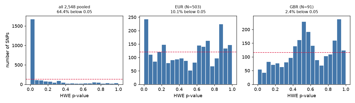
Pooled, 64% of common SNPs reject. Not because 64% of chr22 is broken — because the null is false. Pooling populations with different frequencies produces a heterozygote deficit at every locus in the genome by pure arithmetic. The name for that is the , and the arithmetic above is all of it you need here; Ch 26 §8 and Ch 28, both ahead of you in Part 5, derive it and say what it is good for. The median F of +0.059 is a genome-wide FST readout — the between-group variance ratio S3's worked example put an error bar on — not an assay report. This is why HWE QC must be run within an ancestry-homogeneous stratum, and it is the same phenomenon that forces principal-component covariates into every (Ch 51, S7).
Within EUR the excess is far smaller but not gone — 10.1% against a nominal 5%, and the residual is 1000 Genomes' EUR being itself five populations (GBR, CEU, TSI, IBS, FIN). Within GBR alone the p-values are, if anything, too conservative: only 2.4% fall below 0.05 where 5% should, the small-p end of the histogram is visibly thinned, and the mass has piled up in the middle — 31% of these SNPs land between 0.4 and 0.6, against the 22% a matched null produces. That is not the χ² approximation misbehaving — simulating drawn exactly from HWE at these allele frequencies and N = 91 gives a false-positive rate of 0.046 and a near-flat histogram. It is a property of this dataset: the 1000 Genomes release was genotyped from low- sequencing and then refined using information shared across samples, a step that pulls genotype calls toward population expectations. A p-value histogram that sags at the small-p end and bulges in the middle is itself a finding — flat is what a true null looks like, so a bulge says something upstream regularised your data.
A last caution on this test, and it is the most consequential one in practice. The χ² approximation needs expected counts in every cell, and at low minor- the minor-homozygote expectation is tiny. Compare against plink2 --hardy, which runs the exact conditional test instead:
h = pd.read_csv("labs/data/chr22_hwe.hardy", sep="\t")     # plink2 --hardy, same 2,548 samples
N = G.shape[1]
n0 = (G == 0).sum(1); n1 = (G == 1).sum(1); n2 = (G == 2).sum(1)
p = (2*n0 + n1) / (2*N); q = 1 - p
with np.errstate(all="ignore"):
    F = (n0/N - p**2) / (p*q)
    mine = stats.chi2.sf(N*F**2, 1)
maf, exact = np.minimum(p, q), h["P"].to_numpy()
for lo, hi in [(0.0005, 0.005), (0.005, 0.05), (0.05, 0.5)]:
    m = (maf >= lo) & (maf < hi)
    print(f"MAF [{lo}, {hi}): n={m.sum():6d}  chi2 p<1e-6: {(mine[m]<1e-6).sum():5d}"
          f"   exact p<1e-6: {(exact[m]<1e-6).sum():5d}")
MAF [0.0005,0.005): n= 7312 chi2 p<1e-6: 292 exact p<1e-6: 1
MAF [0.005,0.05): n= 2994 chi2 p<1e-6: 341 exact p<1e-6: 114
MAF [0.05,0.5): n= 2603 chi2 p<1e-6: 824 exact p<1e-6: 793At common frequencies the two agree (824 vs 793). Below MAF 0.5% the χ² test 292 variants that the exact test flags one of — a 292-fold over-rejection, all of it in the anti-conservative direction, all of it good rare variants. Use plink2 --hardy (or --hardy midp) rather than a hand-rolled χ² whenever the minor allele is rare; SciPy has no built-in Hardy–Weinberg exact test.
7. Multiple testing, introduced
Set α = 0.05 and you have declared a willingness to be wrong one time in twenty. Run the test 3,564 times and you have declared a willingness to be wrong about 178 times. The curriculum's QC'd set is exactly 3,564 SNPs in 2,503 unrelated samples, so we can watch it happen — with a that is a coin flip, so every null is true by construction.
qc = pd.read_csv("labs/data/chr22_qc.pvar", sep="\t", comment="#", header=None,
                 names=["chrom","pos","id","ref","alt","filter","info"])
psam = pd.read_csv("labs/data/chr22_qc.psam", sep="\t")
X = G[np.isin(pos, qc["pos"])][:, np.isin(samples, psam["#IID"])].astype(float)

Xc = X - X.mean(1, keepdims=True); ss = np.sqrt((Xc**2).sum(1))
n, m = X.shape[1], X.shape[0]
hits, mins = [], []
for _ in range(500):
    y = rng.integers(0, 2, n).astype(float); yc = y - y.mean()   # a coin flip
    r = (Xc @ yc) / (ss * np.sqrt((yc**2).sum()))
    pv = 2 * stats.t.sf(np.abs(r * np.sqrt((n-2)/(1-r**2))), n-2)
    hits.append((pv < 0.05).sum()); mins.append(pv.min())
hits, mins = np.array(hits), np.array(mins)

print(f"500 random phenotypes, {m} SNPs each")
print(f"  mean hits at p<0.05 = {hits.mean():.1f}   (expected {0.05*m:.1f})")
print(f"  range               = {hits.min()} to {hits.max()}")
print(f"  sd of hit count     = {hits.std():.1f}   (binomial sd if independent = {np.sqrt(m*0.05*0.95):.1f})")
print(f"  median smallest p   = {np.median(mins):.2e}")
print(f"  replicates with any p < 0.05/{m} = {(mins < 0.05/m).sum()}/500")
500 random phenotypes, 3564 SNPs each
mean hits at p<0.05 = 177.8 (expected 178.2)
range = 39 to 507
sd of hit count = 82.5 (binomial sd if independent = 13.0)
median smallest p = 6.17e-04
replicates with any p < 0.05/3564 = 6/500Three things to take from this. First, the expectation is exact: 177.8 against a predicted 178.2, and every one of those "hits" is a phenotype that does not exist. Second, the typical best p-value in a null scan is 6 × 10⁻⁴ — a number that would look publishable on its own and means nothing here, which is why the Bonferroni threshold α/m = 1.4 × 10⁻⁵ exists and why only 6 replicates in 500 produce anything beating it. Third, and least obvious: the spread of the hit count is 83, not the 13 you would get from 3,564 independent tests. These SNPs sit within 1 Mb of each other and are in strong (Ch 29), so they are nowhere near independent. Expectation survives dependence; variance does not. Correlated tests are the reason Bonferroni over-corrects in this 1 Mb window — the effective m here is far below 3,564, so α/m is a stricter threshold than controlling the family-wise error rate actually requires, and the honest fix is a smaller effective m (permutation thresholds, effective-number-of-tests corrections).
Resist promoting that into a law about genotype data, because genome-wide the sign can flip. A genotyping array is not the genome: it is a few hundred thousand chosen positions standing in for about ten million common variants, so each marker also speaks for the neighbours it correlates with and you never measured. Counting the rows in your file then under-states how many questions you asked — by roughly two-fold on a typical array. S7 §2 does this properly: it measures the effective number of independent tests rather than assuming one, and shows the answer moving with the population you measured it in.
Separately, insisting that the probability of even one false positive stay below 0.05 is a brutal target once m is large, which is why false-discovery-rate methods — which control the expected proportion of false positives among your discoveries instead — exist. S7 takes both from here.
8. The garden of forking paths
Multiple testing does not require you to report many tests. It only requires you to have had the option of many, because the effective m is the number of analyses you would have been willing to run, not the number you did run. Every one of the choices below is defensible, and each one is made after seeing data.
Same real , same coin-flip . Now allow three genetic codings (additive, , ) and five populations to analyse separately, and report the best p-value:
codings = {"additive": X, "dominant": (X >= 1).astype(float), "recessive": (X == 2).astype(float)}
sp = panel["super_pop"].to_numpy()[np.isin(samples, psam["#IID"])]
POPS = ["EUR", "AFR", "EAS", "SAS", "AMR"]

def pvals(Xm, y):
    Xc = Xm - Xm.mean(1, keepdims=True); yc = y - y.mean(); n = len(y)
    den = np.sqrt((Xc**2).sum(1) * (yc**2).sum())
    r = np.clip(np.divide(Xc@yc, den, out=np.zeros(Xm.shape[0]), where=den>0), -.999999, .999999)
    return 2 * stats.t.sf(np.abs(r*np.sqrt((n-2)/(1-r**2))), n-2)

res = {k: [] for k in ["additive only", "best of 3 codings", "best of 5 populations", "best of all 15"]}
for _ in range(200):
    y = rng.integers(0, 2, X.shape[1]).astype(float)
    res["additive only"].append((pvals(X, y) < 0.05).mean())
    res["best of 3 codings"].append(
        (np.stack([pvals(v, y) for v in codings.values()]).min(0) < 0.05).mean())
    res["best of 5 populations"].append(
        (np.stack([pvals(X[:, sp==s], y[sp==s]) for s in POPS]).min(0) < 0.05).mean())
    res["best of all 15"].append(
        (np.stack([pvals(v[:, sp==s], y[sp==s]) for v in codings.values() for s in POPS]).min(0) < 0.05).mean())
for k, v in res.items():
    print(f"  {k:24s} type-I error at alpha=0.05 : {np.mean(v):.4f}")
additive only type-I error at alpha=0.05 : 0.0494
best of 3 codings type-I error at alpha=0.05 : 0.0903
best of 5 populations type-I error at alpha=0.05 : 0.1782
best of all 15 type-I error at alpha=0.05 : 0.2676A nominal 5% test now rejects 27% of the time on data with no signal whatsoever, and nobody lied, fabricated, or ran a test they did not believe in. "The effect is recessive." "It's present in Europeans." Both are ordinary sentences in ordinary papers. The defences are pre-registration, an explicit analysis plan, correcting for every path you could have taken, and — the only one that always works — replication in data you had not seen.
9. Where the frequentist frame runs out
Everything above conditions on the null being true and asks about the data. That is a strange direction to reason in, and it is why the misreadings in §3 are so persistent: people keep translating p-values into the statement they wanted, which is about the hypothesis given the data.
Getting that statement legitimately requires a prior over hypotheses, and then Bayes' theorem turns the likelihood into a posterior. The PPV table in §3 was a Bayesian calculation wearing frequentist clothes — "1% of variants are broken" was a prior, and 0.168 was a . Genomics uses the explicit machinery constantly: posterior probabilities in variant callers (Ch 46), posterior probabilities on trees (Ch 34), posteriors (Ch 52), and the ACMG framework for clinical variant classification (Ch 55). That is S6.
Common misconceptions
| What people think | What's actually true |
|---|---|
| p = 0.03 means a 3% chance the null is true | It means data this extreme arise 3% of the time if the null is true. The probability the null is true depends on the base rate — at a 1% prior and α = 0.05, 83% of your rejections are nulls (§3) |
| p = 0.03 means a 97% chance the effect is real | Same reversal, restated. It is the single most common error in the applied literature |
| A non-significant result means no effect | It means the test could not distinguish the data from the null. At N = 91 the HWE test has 7.6% power against F = 0.05 — it would miss almost every real departure (§5) |
| A smaller p means a bigger effect | p mixes effect size with sample size. Report F̂, or a fold change, or an odds ratio, with an interval |
| p = 0.049 and p = 0.051 are different findings | They are the same finding. The 0.05 threshold is a convention, not a discontinuity in nature |
| Three classes means df = 2 | df = 1, because p was estimated from the same counts. Using df = 2 cuts the false-positive rate to 1.4% and throws away power (§2) |
| A conservative test is the safe choice | It is safe against Type I and reckless against Type II. Conservative tests hide real problems, which for a QC filter is the failure that matters |
| α = 0.05 is a law of nature | It is Fisher's arbitrary convenience. Genomics routinely uses 5 × 10⁻⁸, 10⁻⁶, or an FDR target instead, because m is not 1 |
| Chi-square works on any count table | It is an asymptotic approximation. Below MAF ~0.5% it over-rejects HWE by ~300× against the exact test (§6) |
| Testing many hypotheses is fine if you report them all | Reporting is not the issue; the effective m is the number of analyses you could have run. Choosing a genetic model and a subgroup after the fact takes a 5% test to 27% (§8) |
| Correcting for m independent tests is enough | Genotype tests are correlated by LD. The expected number of false positives is unchanged, but its standard deviation is six times larger (§7) |
| If it replicates at p < 0.05 it's confirmed | A replication at 50% power fails half the time when the effect is real, and succeeds 5% of the time when it isn't. Power the replication, or the exercise is theatre |
Worked example: a variant fails HWE at p = 10⁻²⁵. Should you drop it?
chr22:20,711,357 (A>G) in the 503 European-ancestry samples: 306 AA, 109 AG, 88 GG.
Step 1 — compute the statistic and the effect size, not just the p-value. p̂(A) = (612 + 109)/1006 = 0.717. Expected 258.4 / 204.3 / 40.4 against observed 306 / 109 / 88. F̂ = +0.466, χ² = N F̂² = 503 × 0.2175 = 109.4, p = 1.3 × 10⁻²⁵ on 1 df.
Step 2 — check the test is valid. Smallest expected cell is 40.4, MAF is 0.283, N is 503. The asymptotic χ² is fine here; no need for the exact test (§6).
Step 3 — read the sign. F̂ > 0 is a heterozygote deficit: too few AG calls. The candidate explanations are inbreeding, population structure, and — a second variant under a primer or probe site, a null , or an overlapping deletion.
Step 4 — use the structure of the data to discriminate. Population structure is a property of how you pooled; an assay artefact is a property of the assay. So stratify:
| Group | N | AA / AG / GG | F̂ | p |
|---|---|---|---|---|
| EUR | 503 | 306 / 109 / 88 | +0.466 | 1.3 × 10⁻²⁵ |
| AFR | 660 | 116 / 209 / 335 | +0.288 | 1.3 × 10⁻¹³ |
| EAS | 504 | 221 / 119 / 164 | +0.522 | 1.1 × 10⁻³¹ |
| SAS | 489 | 338 / 92 / 59 | +0.442 | 1.4 × 10⁻²² |
| AMR | 347 | 161 / 113 / 73 | +0.304 | 1.5 × 10⁻⁸ |
| GBR | 91 | 54 / 19 / 18 | +0.505 | 1.5 × 10⁻⁶ |
| CEU | 99 | 66 / 16 / 17 | +0.572 | 1.3 × 10⁻⁸ |
Step 5 — conclude. The deficit is the same sign and the same magnitude in every super-population, and survives all the way down to single populations of ~100 people where structure and differ wildly. Structure cannot do that — Wahlund depends on which groups you mixed, and here there is nothing left to mix. An F̂ of +0.5 also has no plausible biological source: Ch 26 §5 will show, in Part 5, that even a fully lethal induces only F = −q. A systematic failure to call heterozygotes does exactly this, and this 1 Mb window sits inside 22q11.2, a region unusually rich in low-copy repeats where mismapping and copy-number variation are common. Drop it, and the region.
Step 6 — note what the p-value contributed. Almost nothing. Every one of those p-values is below 10⁻⁶; they are indistinguishable as evidence and none of them told you the direction, the magnitude, or the cause. The diagnosis came from the sign and stability of F̂ across strata. The p-value's only job was to get the variant onto the list. Its counterpart at chr22:20,833,663 has F̂ between −0.18 and −0.43 in every population — a heterozygote excess, the signature of two paralogues collapsed onto one locus, and a different repair.
Where this is used
- Ch 12 — χ² on progeny counts, estimated-parameter df, and ascertainment as a modelling error
- Ch 26 — the HWE test, the exact test for rare variants, and the power table this chapter derives
- Ch 28 — F and FST, the effect size behind the test in §6
- Ch 33 — Tajima's D, HKA, MK: tests whose null distributions are built by simulation, exactly as in §2
- Ch 46 — HWE and excess-heterozygosity as variant filters
- Ch 47 — tens of thousands of gene-level tests, and why the raw p-value column is never the answer column
- Ch 51 — 5 × 10⁻⁸, , , and replication as the real threshold
- Ch 57 — why clinical reporting thresholds are not statistical thresholds
lab-07andlab-08run these tests on the data used here